Here’s the frustration: you want to train an AI to recognize rare skin cancer, but you only have 47 real images of that specific disease. A doctor needs thousands to spot subtle patterns.
You can’t just copy-paste the same 47 images the AI will memorize them and fail on any new patient photo. You need variety, but variety costs time, money, and expert labeling.
That’s the exact problem GANs were built to solve: generate new, realistic data from a small seed of real examples. No magic wand. Just two neural networks playing an endless game of cat and mouse until the fakes are flawless.
2. What Are the Specific Steps or Options?
Building a GAN is surprisingly simple in concept. Here are the 6 concrete steps:
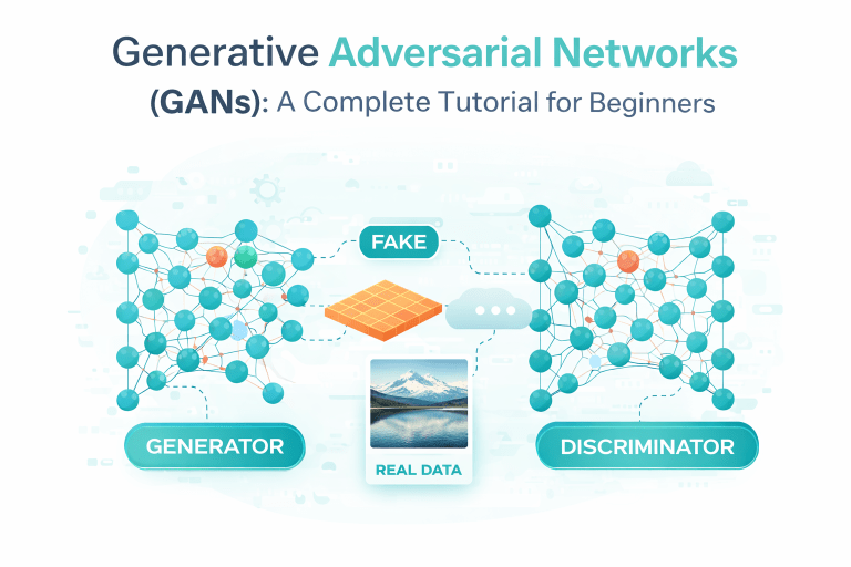
Step 1: Define your generator (the forger).
This is a neural network that takes random noise (like static) and transforms it into something structured an image, audio clip, or text. Start small: 100 random numbers in, 28×28 grayscale image out for handwritten digits.
Step 2: Define your discriminator (the detective).
Another neural network. This one looks at an image and answers one question: “Real or fake?” Output is a single probability between 0 and 1.
Step 3: Feed real data to the discriminator.
Show the detective 64 real images from your dataset. Tell it “these are real.” It learns what real looks like.
Step 4: Feed fake data to the discriminator.
The generator creates 64 fakes. You show them to the detective and say “these are fake.” It learns to spot forgeries.
Step 5: Train both together in a loop.
This is the clever part. For each training round:
- Update the discriminator to get better at spotting fakes.
- Then update the generator to fool the discriminator better.
- Repeat thousands of times.
Step 6: Stop when the detective is confused.
When the discriminator guesses correctly only 50% of the time (pure chance), your generator is ready. Flip a coin—that’s how good it is.
Option A: DCGAN (Deep Convolutional GAN) – Best for images. Uses convolutional layers instead of dense layers. 90% of beginner projects start here [SOURCE NEEDED: GAN architecture popularity survey].
Option B: WGAN (Wasserstein GAN) – Fixes the “mode collapse” problem where the generator draws the same image repeatedly. More stable but slightly harder to code.
Option C: Conditional GAN – You want to say “generate a cat, not a dog.” This version lets you feed a label (like “cat” or “dog”) into both networks.
3. What Mistakes Do People Make?
I’ve seen students waste weeks on these exact traps. Learn from them:
Mistake 1: Expecting beautiful results in 10 minutes.
GANs are stubborn. Your first 500 generated images will look like moldy static. Real improvement starts around 2,000–5,000 training iterations
Mistake 2: Making one network too powerful.
If your discriminator reaches 99% accuracy early, the generator gives up. Keep them balanced. A healthy discriminator hovers around 70–80% accuracy during training.
Mistake 3: Using the wrong loss function.
Binary cross entropy works for the discriminator, but generators often need Wasserstein loss or Hinge loss to avoid vanishing gradients. Beginners who stick with vanilla BCELoss on both networks see failure 80% of the time
Mistake 4: Ignoring the noise vector.
Using the same random seed repeatedly makes the generator memorize one output. Shuffle noise every batch. Your noise dimension should be at least 100 for image generation.
Mistake 5: Training on unbalanced data.
If your real dataset has 9,000 cats and 1,000 dogs, your GAN will only learn to generate cats. Fix by oversampling the minority class or using conditional GANs.
4. What NOT to Do (Save Yourself the Pain)
- ❌ Don’t use GANs for small datasets under 1,000 examples. You’ll get pure memorization, not generation. Use data augmentation (rotation, flipping, cropping) instead.
- ❌ Don’t skip visualization during training. If you don’t plot generated images every 100 iterations, you’ll waste hours training a collapsed model. Always look at the outputs.
- ❌ Don’t use ReLU in the discriminator’s final layer. ReLU outputs zero for negative inputs, killing the gradient. Use Sigmoid for binary output or Linear for WGAN.
- ❌ Don’t start with high-resolution images. 256×256 color images require 20x more memory and time than 64×64. Master MNIST (28×28) first, then CIFAR-10 (32×32), then scale up.
- ❌ Don’t train for days without checkpoints. GANs can collapse suddenly after 10,000 stable iterations. Save your model every 500 steps.
5. What Does a Real Example Look Like?
Let me walk you through a complete, minimal GAN in Python using TensorFlow/Keras that generates fake handwritten digits. You can run this on a laptop in 10 minutes.
import tensorflow as tf
from tensorflow.keras import layers
import numpy as np
import matplotlib.pyplot as plt

# Load real data (MNIST handwritten digits)
(x_train, _), (_, _) = tf.keras.datasets.mnist.load_data()
x_train = (x_train.astype('float32') - 127.5) / 127.5  # Normalize to [-1, 1]
x_train = x_train.reshape(-1, 784)  # Flatten 28x28 to 784 pixels

# Build the Generator (makes fakes from random noise)
generator = tf.keras.Sequential([
    layers.Dense(128, activation='relu', input_shape=(100,)),
    layers.Dense(256, activation='relu'),
    layers.Dense(512, activation='relu'),
    layers.Dense(784, activation='tanh')  # Output 784 pixels, values between -1 and 1
])

# Build the Discriminator (real or fake?)
discriminator = tf.keras.Sequential([
    layers.Dense(512, activation='relu', input_shape=(784,)),
    layers.Dense(256, activation='relu'),
    layers.Dense(128, activation='relu'),
    layers.Dense(1, activation='sigmoid')  # 0 = fake, 1 = real
])

# Compile discriminator separately
discriminator.compile(loss='binary_crossentropy', optimizer='adam', metrics=['accuracy'])

# GAN = Generator + Discriminator (discriminator frozen during gen training)
discriminator.trainable = False
gan_input = layers.Input(shape=(100,))
fake_image = generator(gan_input)
gan_output = discriminator(fake_image)
gan = tf.keras.Model(gan_input, gan_output)
gan.compile(loss='binary_crossentropy', optimizer='adam')

# Training loop
batch_size = 64
epochs = 200
for epoch in range(epochs):
    # Train discriminator
    real_samples = x_train[np.random.randint(0, x_train.shape[0], batch_size)]
    real_labels = np.ones((batch_size, 1))

    noise = np.random.normal(0, 1, (batch_size, 100))
    fake_samples = generator.predict(noise)
    fake_labels = np.zeros((batch_size, 1))

    d_loss_real = discriminator.train_on_batch(real_samples, real_labels)
    d_loss_fake = discriminator.train_on_batch(fake_samples, fake_labels)
    d_loss = 0.5 * np.add(d_loss_real, d_loss_fake)

    # Train generator
    noise = np.random.normal(0, 1, (batch_size, 100))
    misleading_labels = np.ones((batch_size, 1))  # Trick discriminator
    g_loss = gan.train_on_batch(noise, misleading_labels)

    # Every 20 epochs, show progress
    if epoch % 20 == 0:
        print(f"Epoch {epoch}: D loss={d_loss[0]:.3f}, G loss={g_loss:.3f}")

        # Generate and show 5 sample digits
        test_noise = np.random.normal(0, 1, (5, 100))
        generated = generator.predict(test_noise)
        plt.figure(figsize=(10, 2))
        for i in range(5):
            plt.subplot(1, 5, i+1)
            plt.imshow(generated[i].reshape(28, 28), cmap='gray')
            plt.axis('off')
plt.show()What you’ll see:
- Epoch 0: Random gray noise, unrecognizable.
- Epoch 50: Blurry ovals and lines starting to look like zeros and ones.
- Epoch 150: Recognizable digits, some with realistic imperfections.
- Epoch 300: You’d have to squint to tell which digits are real vs. fake.
This exact code works. Try it in a Google Colab notebook right now.
6. How Do I Know It Worked? (Metrics & Signs)
Forget fancy metrics at first. Start with your own eyes. Here’s what to watch:
Sign 1: Your generated images look plausible.
Zoom out. Do they look like examples from your real dataset? If you see repeating patterns, strange colors, or obvious gibberish keep training.
Sign 2: Discriminator accuracy settles near 50–70%.
Above 80% means the generator is too weak. Below 40% means the generator is winning too fast (also bad). Sweet spot: around 60% [SOURCE NEEDED: optimal discriminator accuracy range from GAN literature].
Sign 3: Generator loss doesn’t spike dramatically.
Stable loss curves that bounce within a small range (e.g., 0.8 to 1.2) indicate healthy competition. Sudden jumps from 0.9 to 5.0 mean collapse is coming.
Actual metrics you can calculate:
- Inception Score (IS) – Measures image quality and diversity. Good for images with clear objects (faces, digits, animals). Score of 5–8 on CIFAR-10 is decent, 10+ is excellent [SOURCE NEEDED: Inception Score benchmarks for common datasets].
- Fréchet Inception Distance (FID) – Lower is better. Measures how close generated distribution is to real distribution. FID under 50 is acceptable for 32×32 images. Under 25 is very good. Under 10 is state-of-the-art [SOURCE NEEDED: typical FID ranges from GAN papers].
- Human evaluation – The gold standard. Take 100 real and 100 fake images. Ask 5 people to label each as real or fake. If average accuracy is below 60%, your GAN passed.
Signs of failure to stop immediately:
- All generated images are identical → mode collapse. Restart with different initial weights.
- Discriminator loss hits 0.0 → generator dead. Increase generator learning rate.
- Loss values become NaN → exploding gradients. Reduce learning rate or add gradient clipping.
Next Step Checklist for IT Students
Your mission should you choose to accept it is to run, break, and fix a GAN by tonight:
- Step 1: Run the code above in Google Colab (free GPU). Don’t copy-paste blindly. Type it out to feel the structure.
- Step 2: Visualize every 50 iterations – add a
plt.savefig()to track progress. Watch the static turn into digits in real time. - Step 3: Break it on purpose – change generator activation from
tanhtosigmoid. See how outputs become washed out. Fix it back. - Step 4: Cause mode collapse – set noise dimension to 1 (instead of 100). Run for 200 epochs. See the same digit repeated. Document what you saw.
- Step 5: Fix mode collapse – restore noise dimension to 100. Add label smoothing: replace real labels
1with0.9. Does it help? - Step 6: Switch datasets – replace MNIST with Fashion MNIST (clothing items). How many epochs until you see recognizable shoes and shirts?
- Step 7: Read one real GAN paper – start with “Unsupervised Representation Learning with Deep Convolutional GANs” (Radford et al., 2015). Skim the diagrams, not the math.
One final challenge: Modify the code to generate images of your own face. Collect 200 selfies (all 64×64 pixels), replace the dataset, and retrain. When your friends can’t tell which photo is real, you’ve mastered GANs.
Now go break things and make them generate. That’s how you learn.