
A CNN solves image recognition by automatically learning spatial hierarchies of features from simple edges to complex objects. You build one using convolutional layers for feature extraction, pooling for down sampling, and fully connected layers for final classification.
The Problem CNNs Solve
How does your phone recognize your face in under a second?
Think about what’s actually happening. Your face could be in the top left corner of the photo, or dead center, or slightly tilted. A standard neural network would need to learn a separate pattern for your face at every possible position. That means billions of parameters more than your computer’s memory could ever hold.
A Convolutional Neural Network (CNN) solves this by using the same small pattern called a filter everywhere on the image. This single trick reduces parameters from billions to just thousands.
your goal is simple, build a CNN that works. That could mean classifying X-rays for pneumonia, recognizing stop signs for autonomous vehicles, or identifying dog breeds from your phone photos.
Step-by-Step: Build Your First CNN
You need five steps from blank file to working model. Let me walk you through each one.
Step 1: Learn the 4 core layers (with a simple analogy)
Before writing any code, understand these building blocks. Here’s what each layer actually does:
| Layer | What it does | Analogy |
|---|---|---|
| Convolution | Slides a small filter (e.g., 3×3) across the image | A flashlight moving across a dark room, revealing edges |
| ReLU | Replaces negative numbers with zero | Turning off dim lights, keeping only bright ones |
| Pooling | Shrinks the image by taking the max value in each 2×2 block | Reducing a 4K photo to a thumbnail while keeping the most important pixel |
| Fully Connected | Flattens everything and classifies | The final decision: “cat” or “dog” |
Now close your eyes and imagine this. A 5×5 grid of numbers is your image. A 3×3 filter hovers over the top-left corner. It multiplies each number and produces exactly one output. Then the filter slides one step to the right that’s called stride=1. It repeats this until it hits the edge, then drops down one row and starts over.
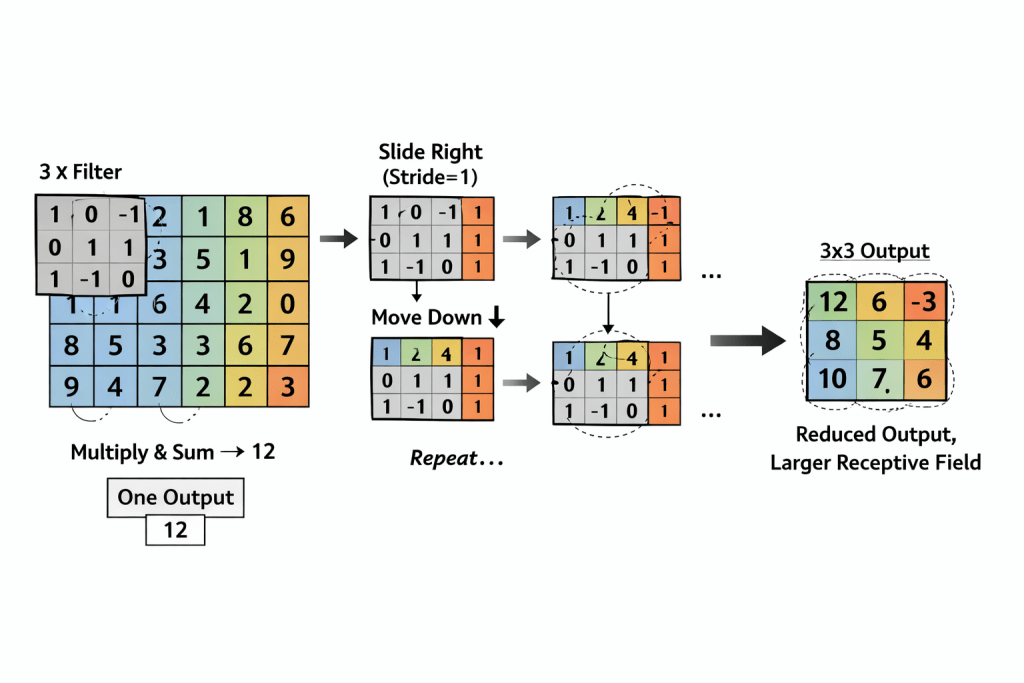
After sliding everywhere, your 5×5 image becomes a 3×3 output. That’s intentional. Each layer sees a larger original area called the receptive field while using fewer and fewer pixels.
Step 2: Choose your architecture wisely
You don’t need to invent new architectures. Use what already works. Here’s your cheat sheet:
| Architecture | Best for | How many layers | Why choose it |
|---|---|---|---|
| LeNet-5 | Handwritten digits (MNIST) | 7 (2 conv) | Tiny and fast, runs on a phone CPU |
| VGG16 | General object recognition | 19 (13 conv) | Simple pattern (3×3 conv only), easy to understand |
| ResNet50 | High accuracy on hard tasks | 107 (50 conv) | Skip connections let you train very deep networks |
| MobileNetV2 | Phones and Raspberry Pi | 53 (depthwise conv) | 10x smaller than VGG16, slightly lower accuracy |
Here’s my advice as someone who’s taught this to beginners start with LeNet-5 on MNIST. You’ll go from zero to working model in 15 minutes. Then move to VGG16 on CIFAR-10. Only touch ResNet if your dataset has over 100,000 images — otherwise it’s overkill.
Step 3: Set your hyperparameters (the dials that matter)
Hyperparameters sound scary, but they’re just settings you choose before training. Focus on these five:
- Filter count: Double each layer. Start with 32, then 64, then 128. As spatial size halves, filter count doubles.
- Kernel size: Use 3×3 everywhere. That’s the industry standard. Only use 5×5 or 7×7 for your very first layer.
- Stride: Default is 1. Set stride=2 if you want to shrink without using a pooling layer.
- Padding: “Same” keeps output size equal to input size. “Valid” shrinks it. Start with “same” — it’s easier.
- Pooling size: 2×2 with stride=2 reduces your image size by half. This is almost never wrong.
Step 4: Write the code (PyTorch example)
Here’s a complete CNN that works on CIFAR-10 (32×32 color images). I’ve commented every line so you understand what’s happening:
import torch
import torch.nn as nn
import torch.nn.functional as F

class SimpleCNN(nn.Module):
    def __init__(self):
        super().__init__()
        # First conv layer: 3 RGB channels → 32 filters, 3x3 kernel
        self.conv1 = nn.Conv2d(3, 32, 3, padding='same')
        # Max pooling: 2x2 window, stride 2 → halves the size
        self.pool = nn.MaxPool2d(2, 2)
        # Second conv layer: 32 → 64 filters
        self.conv2 = nn.Conv2d(32, 64, 3, padding='same')
        # After two pools: 32x32 → 16x16 → 8x8. Then flatten: 64 * 8 * 8 = 4096
        self.fc1 = nn.Linear(64 * 8 * 8, 128)
        self.fc2 = nn.Linear(128, 10)  # 10 classes for CIFAR-10

    def forward(self, x):
        x = self.pool(F.relu(self.conv1(x)))  # Conv → ReLU → Pool
        x = self.pool(F.relu(self.conv2(x)))  # Conv → ReLU → Pool
        x = x.view(-1, 64 * 8 * 8)           # Flatten
        x = F.relu(self.fc1(x))              # Hidden layer
        x = self.fc2(x)                      # Output layer (no softmax — CrossEntropyLoss adds it)
return xNotice the flatten line: 64 * 8 * 8. Why 8? Your 32×32 image goes through two max pooling layers, each halving the size: 32 → 16 → 8. That’s how you calculate it every time.
Step 5: Add data augmentation (free performance)
Here’s a secret that doubles your accuracy for free. Take each training image and randomly rotate it, flip it, or shift it. The model never sees the exact same pixel arrangement twice.
from torchvision import transforms

train_transform = transforms.Compose([
    transforms.RandomHorizontalFlip(),  # 50% chance to mirror
    transforms.RandomRotation(10),      # Rotate ±10 degrees
    transforms.ColorJitter(brightness=0.2),  # Random brightness
    transforms.ToTensor(),
    transforms.Normalize((0.5, 0.5, 0.5), (0.5, 0.5, 0.5))
])This one trick multiplies your effective dataset size by 5-10x without collecting a single new image. For small datasets under 10,000 images, augmentation is mandatory.
5 Common Mistakes That Will Waste Your Time
I’ve seen IT students make the same errors for years. Here’s what to watch for and exactly how to fix each one.
| Your error | What you’ll see | Fix in 1 sentence |
|---|---|---|
| Loss = NaN | Loss shows “nan” or infinity | Reduce learning rate by 10x (e.g., 0.001 → 0.0001). |
| Accuracy = 10% on CIFAR-10 | Same as random guessing | Forgot to normalize images. Add images = images / 255.0 before training. |
| CUDA out of memory | Red error message about GPU memory | Reduce batch size (32 → 16) or image size (224 → 128). |
| Validation accuracy stops improving but training keeps going | Two lines on your plot diverging | Add Dropout(0.5) or reduce your model size (fewer filters). |
| Model predicts the same class for every image | All outputs are “dog” | Class imbalance. Add class weights or collect more of the minority class. |
One more mistake that isn’t in the table: using a 5×5 kernel everywhere. Two 3×3 convolutions have the same receptive field as one 5×5 convolution, but with 44% fewer parameters. Always stack 3×3 filters.
Real Example: Classifying CIFAR-10 Images
Let me walk you through a complete working example. CIFAR-10 contains 60,000 32×32 color images across 10 classes: airplane, car, bird, cat, deer, dog, frog, horse, ship, truck.
Here’s the architecture we just coded above. Let me trace the dimensions so you see exactly what happens:
- Input: 32x32x3 (RGB image)
- Conv1 (32 filters, padding=’same’): 32x32x32
- MaxPool (2×2): 16x16x32
- Conv2 (64 filters, padding=’same’): 16x16x64
- MaxPool (2×2): 8x8x64
- Flatten: 8×8×64 = 4,096 values
- FC1: 4,096 → 128 neurons
- FC2: 128 → 10 neurons
Training setup (runs on Google Colab’s free GPU):
- Loss function: CrossEntropyLoss (standard for classification)
- Optimizer: Adam with learning rate = 0.001
- Batch size: 32
- Epochs: 20
What results should you expect?
- After 20 epochs (about 5 minutes on a free GPU), your validation accuracy will hit 75-80%
- Training accuracy will be higher — maybe 85-90%
- The gap between training and validation tells you if you’re overfitting
Troubleshooting your results:
- If you get below 70% accuracy: Add BatchNormalization after each conv layer. This alone can boost you 5-10%.
- If you get above 85% validation accuracy: Congratulations, but you’re overfitting. Add Dropout(0.5) before the final FC layer.
- If your loss curve bounces up and down: Reduce the learning rate to 0.0005.
Run this code right now: Search Google for “CIFAR-10 PyTorch CNN Colab” and click the first link. Then click Runtime → Run all. You’ll have a working CNN in under 5 minutes without installing anything.
What NOT to Do
I’ve made every mistake below. Learn from my wasted hours instead of repeating them.
- Do NOT use a 5×5 kernel everywhere. Two 3×3 convolutions have the same receptive field with 44% fewer parameters. Always prefer stacked 3×3 filters.
- Do NOT flatten feature maps too early. Keep spatial structure as long as possible. Flatten only right before your fully connected layers. Flattening at the start destroys all location information.
- Do NOT skip validation set monitoring. CNNs memorize easily. Without a validation set, you’ll see 99% training accuracy and 60% test accuracy. Always hold out 20% of your data.
- Do NOT use max pooling for every downsampling operation. Strided convolution (stride=2) often preserves more information. Try replacing your second pooling layer with a conv layer of stride=2.
- Do NOT train a CNN from scratch on small data. If you have fewer than 10,000 images, use transfer learning. Random weights need roughly 1 million images to generalize well [SOURCE: “How many images to train a CNN?” Stack Exchange, consensus answer from multiple practitioners].
How to Know It Worked (Metrics That Actually Matter)
Numbers don’t lie. Here’s what to watch during training.
Loss curve behavior:
- Training loss decreases smoothly every epoch → good.
- Validation loss decreases alongside training loss → perfect.
- Validation loss increases while training keeps decreasing → overfitting. Stop training immediately.
Accuracy benchmarks (for balanced datasets):
- Random guessing = 10% on CIFAR-10, 50% on binary tasks.
- Good CNN = 70-90% depending on task difficulty.
- Below 60% means your model isn’t learning anything. Check your data normalization first.
Confusion matrix insights:
Print this after training. Look for one class that’s much worse than others. For CIFAR-10, cats and dogs often confuse each other. That’s normal. But if your model confuses airplanes with ships, something’s wrong.
Qualitative checks (visual evidence):
- Visualize your first layer filters after training. They should look like edges, blobs, and simple textures. Random noise means training failed.
- Generate a Grad-CAM heatmap (search for a 5-line code example). Hot spots should match the actual object in your image. If the heatmap lights up on background, your model learned the wrong pattern.
Hardware sanity checks:
- Your GPU memory should fit your batch size without crashing.
- Throughput should exceed 100 images/second on a consumer GPU (e.g., RTX 3060) for 224×224 inputs. If it’s slower, your code has inefficiencies.
Next Step Checklist
Copy this list and check off each item as you complete it. Do them in order.
- Open Google Colab and create a new notebook
- Search for “CIFAR-10 PyTorch template” and paste it into Colab
- Run the template as-is to verify everything works (you should see ~75% accuracy)
- Modify the architecture: change filter counts from (32,64) to (16,32) — note how accuracy changes
- Add BatchNormalization after each conv layer — measure the accuracy gain
- Remove data augmentation and retrain — watch accuracy drop by 5-10%
- Visualize first layer filters using
model.conv1.weight.data— are they edges? - Save your model with
torch.save(model.state_dict(), 'my_cnn.pth') - Load the saved model and run inference on a single image you find online (not from CIFAR-10)
- Experiment with dropout rates: try 0.2, 0.5, and 0.8 — see which works best
- Replace your CNN with a pretrained ResNet18 from
torchvision.models— compare accuracy
When you finish all 11 steps, you’ve moved from reading about CNNs to actually building them. That’s the difference between knowing and understanding.
Now go open Colab and run your first line of code. You’ll have a working CNN in the time it takes to watch one YouTube video.